From Words to Vectors: The Journey of Word Embeddings

Have you ever wondered how AI models like Chat GPT and Gemini see words and sentences? Well, just like everything with AI, it’s all numbers! Words and sentences are converted to “vectors” before being passed to AI models. Vectors, if you’re not familiar with them, are just a list of numbers. As we shall see in this post, current AI models represent each word in human language by a unique list of numbers, but where it gets REALLY interesting is that the AI learns those numbers for every word completely on its own. You just have to give it a ton of data, and by data, we’re talking about a large corpus of human text, such as all of Wikipedia for example.

Types of Embeddings

This blog post will mostly focus on Word and Document embedding. However, the idea of embeddings applies to so much more. Embeddings, in general, are a way to convert some object, such as a word, sentence, or even an image into a vector. There are many types of embeddings and different approaches for each. This list is only a small example of the many kinds of embeddings that exist out there:

• Word Embeddings
  Numerical representations of words capture semantic relationships, allowing computers to understand and process language.
  
• Document/Sentence Embeddings
  Document/sentence embeddings extend the concept of word embeddings to represent entire documents or sentences as single vectors. These embeddings capture the overall meaning and context of the text. These embeddings help in tasks like semantic search, document clustering, and text summarization.
  
• Image Embeddings
  Image embeddings are numerical representations of images, mapping them to dense vectors in a high-dimensional space. These vectors capture an image's features, such as color, texture, and shape.
  
• Graph Embeddings
  Graph embeddings are numerical representations of nodes in a graph, mapping them to dense vectors in a low-dimensional space. These vectors capture the structural and semantic relationships between nodes in the graph.

What are Word Embeddings?

Well, word embeddings mean converting a word into a vector. To be more Mathematically precise, we’re mapping, or “embedding”, each word to some vector in a d-dimensional vector space, where d is the dimension of the vector and is the same for all words. For example, if each word gets mapped to a list of 300 numbers, our word embeddings convert each word to a vector in a 300-dimensional vector space. But how exactly do those mappings work? Well, let’s dive deeper!

How Word Embedding Works

Word embedding begins by training a model on a large text dataset, like Wikipedia. First, the text is preprocessed to ensure the quality. This involves splitting the text into individual words, a step known as tokenization, and removing unnecessary elements such as stop words, punctuation, and special characters.

During training, the model learns to assign a vector to each word, placing words with similar meanings closer together in a shared vector space. By this, word embeddings capture both the unique meaning of each word and the relationships between them, reflecting how they are used. This highlights the strength of word embeddings in positioning words that share meanings or contexts near each other, making it easier to understand the relationships between concepts.

Approaches to word embeddings

1. Frequency-based Approaches

These approaches depend on the occurrences and the word frequency to build vector representations, such as:

1. One Hot Encoding
2. Bag of Words (BoW)
3. Co-occurrence Counts
4. Term Frequency-Inverse Document Frequency (TF-IDF)

2. Prediction-based Approaches

These approaches learn word embeddings by predicting word occurrences based on their context, such as:

1. Word2Vec
2. GloVe (Global Vectors for Word Representation)
3. BERT

Which techniques create word embeddings?

A) Word2Vec and GloVe
B) Word2Vec and FastText
C) TF-IDF and LDA
D) K-Means and PCA

One Hot Encoding

This is the most basic technique to embed words, but as we shall see, it has many disadvantages. To understand this technique more concretely, let’s assume we will choose to set the vocabulary, that is all the words our AI model will ever know or ever have to deal with, to be the 50,000 most common words in the English language. One idea is to sort the words by any order and assign each word a number between 1 and our vocab size, which is 50,000 in this case. Notice how we’ve already converted each word into a number? The next step is to represent each word by a list of numbers of length 50,000 that is all 0’s with a single 1 at the number associated with our target word. In the figure below, the words are sorted alphabetically, and the word Apple is assigned the number 1, for example. The vector associated with Apple is equal to 1 only at the first index with all the other values equal to 0 elsewhere. On the other hand, the last word in our vocab, Zoo, has a corresponding vector that is only equal to 1 at the last index and equal to 0 elsewhere.

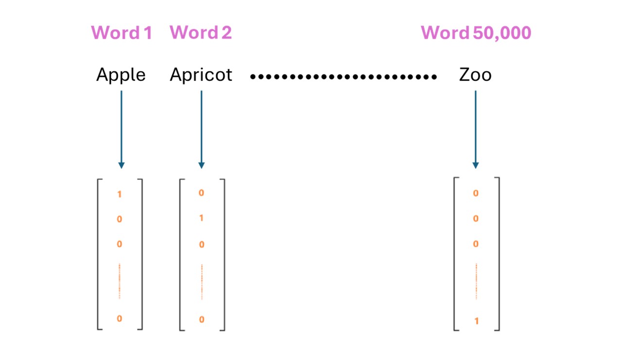
But why are hot encodings a bad idea? Well, there are a couple of problems with this approach:

1. The Vector Dimension is too large = Vocab Size.
   
   
2. The Vectors are sparse, “mostly empty”. Even though we’re using many dimensions per word, we’re wasting most of our vector dimensions by setting them to 0. We’re only making use of 1 single dimension per word when we set it equal to 1.
   
   
3. All words are equally distant in our vector space. As we shall see later on, other techniques for word embeddings have an interesting property in that words with similar meanings get embedded by vectors that are closer to each other.
   
   

Bag Of Words (BOW)

A very similar technique to one-hot encoding used to embed a document, instead of a single word, is known as Bag of Words. When embedding a document with a bag of words, we’re essentially getting the one-hot encoding of every word in the document and summing them all into one single vector representing the document, thus the text is defined as the frequency of words in a document while ignoring the order. The next figure shows how a bag of words would work for 3 sentences, each representing a different document, and a vocab size = 4:

Source: 4 — Bag of Words Model in NLP

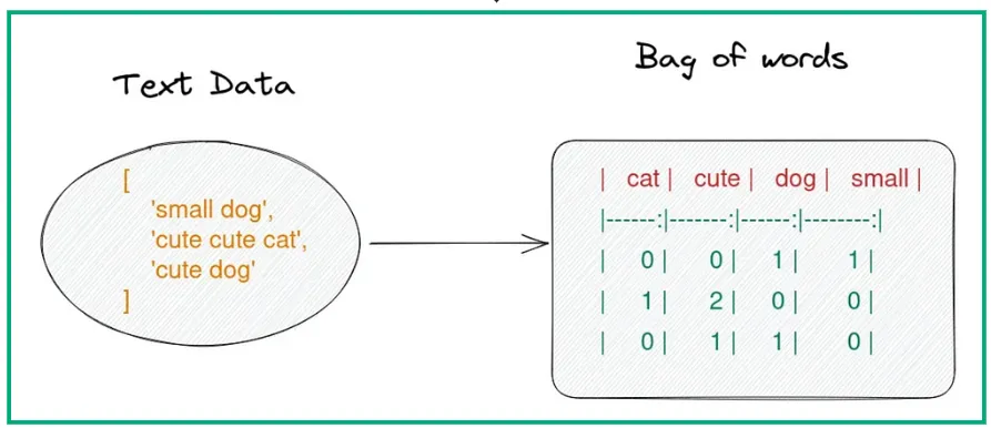
It provides a more compact representation than one-hot encoding but still lacks context and semantic meaning. Each position in the vector corresponds to a word in the vocabulary, in the order they were listed.

Disadvantages:

1. Similar to one-hot encoding, the vector dimension is still too large = Vocabulary Size.
   
   
2. Similar to one-hot encoding, the Bag of Words will still be mostly empty. While the vector in Bag of Words wouldn’t be as empty as with One-Hot-Encoded words, it will still have many unused dimensions in our vector set to 0. For a bag of words to ever have a vector that isn’t mostly empty, it needs to have a TON of words. For example, if we want more than half of our vector to not be set to 0, then we need the encoded document to have half of ALL the words in our vocabulary. For a vocab size = 50,000, we would need our document to have at least 25,000 unique words. However, this will usually not be the case for any document we’re dealing with, so we will end up with mostly empty vectors.
   
   
3. Completely ignores the order. This disadvantage is related to the problem of embedding documents rather than embedding a single word, it is an important problem that appears whenever we try to embed a document as the sum of embeddings for the words in that document.
   
   

Co-occurrence counts

Another way to embed words is by using a co-occurrence matrix. By measuring how often each word occurs with other words we can find a suitable representation of those words. In the next figure, for example, we can see that the word “digital” occurs with “computer” 1670 times, which is way more than “cherry” and “computer” for example. We can use this technique to embed the words by the counts in their corresponding rows.

Source: Vector Semantics and Embeddings (Stanford University) Words Model in NLP

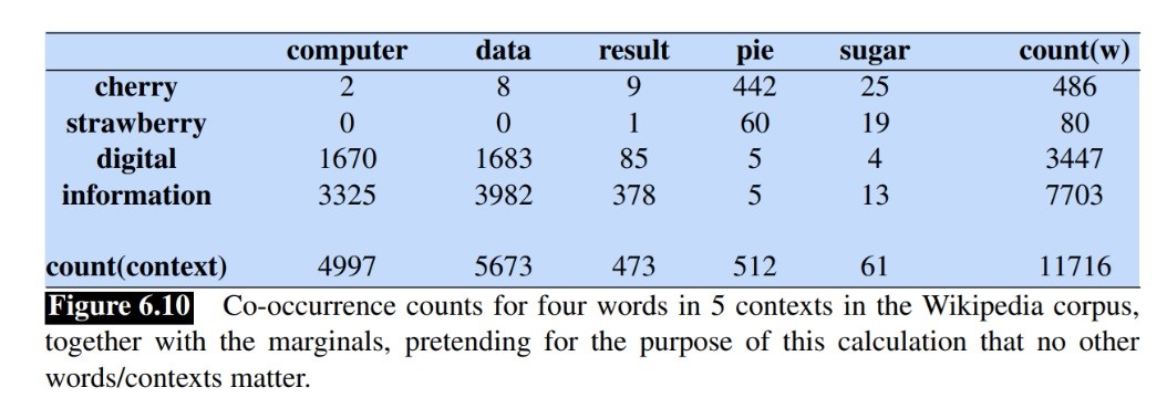
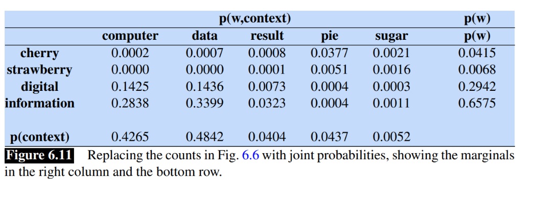
Additionally, we can normalize the counts by dividing them by the total count. For example, in the cherry row, we can divide all counts by 486 to obtain probabilities.

Source: Vector Semantics and Embeddings (Stanford University) Words Model in NLP

Term Frequency-Inverse Document Frequency (TF-IDF)

TF-IDF is a statistical measure used to evaluate the importance of a word in a document relative to a collection of documents. It's commonly used in information retrieval and text mining to help rank the relevance of documents based on keyword searches. It works by essentially measuring, for every word, how much more commonly it occurs in the specific document we are embedding relative to other documents in our data. A term like the word “the”, which could appear a lot in our document but also appears in every other document does not mean much. However, a scientific article with the term “DNA” that frequently appears in that article, but does not frequently appear in general within other documents in our text will likely be a much more powerful measure of the meaning of our document.

Disadvantages:

1. Lack of semantic understanding as it treats words as individual units ignoring their meaning and it doesn't understand the meaning of words in different contexts.
   
   
2. Ignoring word order results in the loss of important contextual information.
   
   
3. TF-IDF vectors can be very sparse like One Hot Encoding, especially for large vocabularies, leading to inefficiencies in storage and computation.
   
   
4. Synonymous words are treated as distinct, even though they have the same meaning, leading to redundancy and lower-quality features.
   
   
5. It gives weight to words based on how often they appear in a document and how rare they are. But it struggles with stopwords and common words like “the,” “and,” or “is” because these words show up a lot but don’t add much meaning so this makes it harder for models to find the important patterns in data.
   
   

Mathematics Behind Word Embeddings

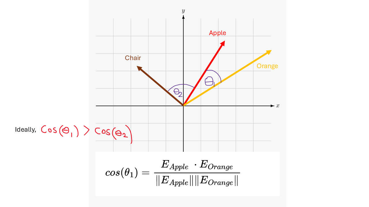
To understand word embeddings better, let’s look at them in a more indepth way. When creating word embeddings, we want to position similar words close to each other in a high-dimensional space, which helps in understanding their meanings and relationships. The main method used to measure this notion of “closeness” in a high dimensional space is the "cosine similarity", which calculates the direction and magnitude of word vectors. To find cosine similarity, we calculate the dot product of two vectors, the sum of the products of their corresponding components, and then normalize by their norms. A higher dot product means stronger relationships between the words. In the following figure for example, ideally, we want the angle between our learned embedding vectors for Apple and Orange to be smaller than the angle between Apple and the Chair, thus the cosine similarity should be higher in the case of Apple and Orange than in Apple and Chair.

What does cosine similarity measure?

A) The Euclidean distance between two points.
B) The angle between two vectors.
C) The average of two vectors.
D) The length of the longest vector.

Word2Vec

Word2Vec is a technique for converting words into dense vectors. It aims to represent words in a continuous vector space, where semantically similar words are mapped to nearby points. These vectors capture information about the words based on the words around them. Word2Vec uses two main approaches:

1. Continuous Bag of Words (CBOW):

It works by predicting the target word using the surrounding context words For example, ”I am drinking ….” Here, CBOW works on figuring out the sentence's meaning and predicting the target word which in this example can be tea.

So, let's dive into the architecture behind CBOW

• Input Layer: In this layer, words are represented by one-hot encoded vectors, where each element in the vector corresponds to a specific word in the vocabulary. For example, if the vocabulary contains 30,000 words, the input layer will have 30,000 elements.
  
• Hidden Layer: In this layer, the word embeddings are formed by getting the average and converting it into a lower-dimensional dense vector. This dense layer has neurons that correspond to each word in the vocabulary. The total number of neurons in the hidden layer equals the number of words in the vocabulary.
  
  
• Output Layer: In this layer, the model uses a softmax function to predict the target word by figuring out which has the highest probability (most likely the middle word) from the vocabulary.
  

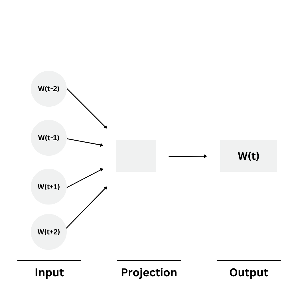
Previously we talked about Bag Of Words (BOW) so, let's know the main differences between CBOW and BOW Each of the BoW and CBOW models serves distinct purposes in natural language processing. BoW represents a document as a collection of words, providing an effective representation by ignoring their order and grammar, and focusing on the frequency of each word. This results in high-dimensional and sparse feature vectors. In contrast, CBOW is a neural network model that predicts a target word based on its surrounding context words, capturing semantic relationships by considering the context in which words appear and identifying the relationships between them.

2. Skip-Gram:

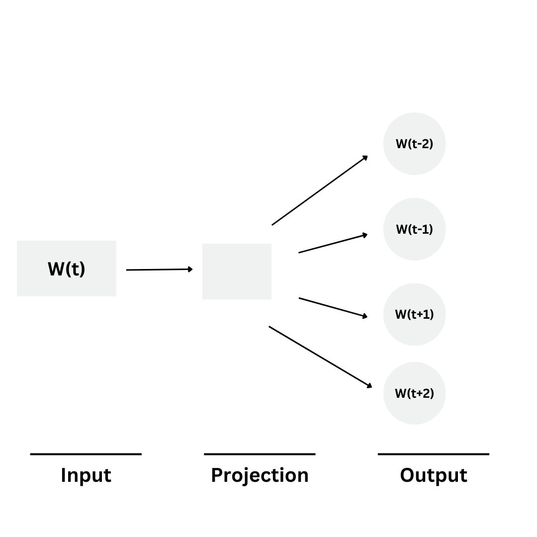
The Skip-gram model is a neural network-based approach for learning word embeddings from a large corpus of text. The main goal of the Skip-gram model is to predict the context words surrounding a target word.

For example: "I am drinking coffee in the morning," the target word could be "drinking." So, Skip-Gram will predict "I," "am," "coffee," and "in."

So, let's dive into the architecture behind Skip-Gram. Firstly, Skip-Gram maintains two vector embeddings, each of the same dimension for each word. If the embedding dimension we’re using is equal to 100, then for each word, we have a 100-dimensional vector that is used when the word is a context word and another 100-dimensional vector that is used when the word is a target word.

You might be wondering why we use two embeddings per word. Well, here's the reasoning:

1. Firstly: In skip-gram, each word can appear as a central (target) word or as a neighboring (context) word around other targets. We want the model to learn not only how the target word itself behaves but also how it influences the words around it. Using separate embeddings for the target and context enables the model to capture these nuanced relationships better.
2. Additionally: Language often has asymmetrical relationships, where the influence of one word on another is not identical when reversed (e.g., "doctor" and "hospital" have different roles when "doctor" is the target vs. "hospital"). By using separate embeddings, skip-gram can learn more refined relationships and better capture the directional context.

Step 1 (Build our Dataset):

To build our dataset from a set of English sentences, we first choose a context window length = 4 for example. Then for every sentence, for every word, treat it as a target word and treat the 4 words before and after it as context words. Add each one of those context/target pairs independently into our dataset. The result of this for a sentence, such as “This is an example sentence in our corpus” will be:

• (This, is) (This, an) (This, example) (This, sentence)
• (is, This) (is, an) (is, example) (is, sentence)
• (an, This) (an, is) (an, example) (an, sentence) (an, in) (an, our)

Where the first word in each parenthesis is the target word and the second word is the context word.

Step 2 (Sample a Pair):

Randomly choose a target/context pair from our dataset.

Step 3 (Embed the pair):

Get the word embedding from our target embedding matrix for the target word, and the word from our context matrix for the context word. Notice that we have two embedding matrices in this case; one that is used when the word is a target word and another that is used when it's a context word.

Notice that we initialize the embedding matrices randomly, so initially those embeddings won’t mean much. However, the word2vec algorithm, given some data, will work on making the embeddings for the words that occur together in the same sentence become more similar.

Step 4 (Calculate the loss):

Intuitively, what this next step is trying to do is “push” the target word embedding closer to the context word embedding, while “pushing” them away from all other context word embeddings. To do this, we calculate the dot product between our target word’s vector embedding and every other context word embedding. Ideally, we want the dot product between our target word and the word that came in its context to be much larger than the dot product between our target word and any other word. In this case, we use a softmax on the resultant dot products and use a cross-entropy loss on the outputs of the softmax. Mathematically, we can represent this by the next equation (where u is the target embedding, v is the context embedding, V is the vocabulary size, and y is the loss):

Source: COS 484 PrincetonLectures: Lecture 5

Have you noticed any problems with this approach? Well, it works well in theory but in practice is very slow. This is because every update to our embeddings requires calculating the dot product between our target word vector and the context embedding for each word in our vocabulary and updating each of those context embeddings. The authors solve this problem using Negative Sampling.

Negative Sampling:

The previous algorithm can be thought of as using every other word that is not our context word as a negative sample for our positive target/context pair. To mitigate this, the authors instead randomly sample 5-20 words at random and treat them as negative samples. In this case, the authors use the sigmoid function instead of the softmax. For the positive sample, the sigmoid is trained to output 1 and for the negative samples, the sigmoid is trained to produce a zero.

The loss is then represented by:

Source: COS 484 PrincetonLectures: Lecture 5

Where Vc is the positive sample and all Vj are the negative samples. Therefore, the negative sampling process can be seen as an alternative way to train our model without having to update all the context words in our vocabulary at every step.

1. In SkipGram with negative sampling, how many parameters are updated for every context/target pair (t,c) where K = Number of negative samples?

A) K x d
B) 2 x K x d
C) (K+1) x d
D) (K+2) x d

2. How many parameters does SkipGram have? (d = embedding dimension, |V| = vocab size, m = context window)

A) d x |V|
B) 2 x d x |V|
C) 2 x m x |V|
D) 2 x m x d x |V|.

GloVe (Global Vectors for Word Representation)

GloVe is a popular algorithm for creating word embeddings. Unlike Word2Vec, GloVe uses the overall co-occurrence patterns of words across the entire text corpus to learn word relationships.

GloVe embeddings are a type of word embedding model designed to capture both the local context and the global statistical information of words in a corpus. Developed by researchers at Stanford, GloVe learns word representations by constructing word co-occurrence matrices from large text corpora, capturing meaningful patterns in word usage. By focusing on ratios of word co-occurrences rather than individual occurrences, GloVe embeddings effectively capture semantic relationships between words, such as similarity and analogy (e.g., "king" - "man" + "woman" ≈ "queen"). GloVe embeddings are widely used in NLP tasks, as they provide dense, meaningful representations that enhance machine learning models’ understanding of language .

GloVe works by first collecting large text data from sources like Wikipedia or news articles. It then builds a co-occurrence matrix, which records how often pairs of words appear close to each other within a certain window. This matrix helps the model capture relationships between words based on their context. For example, if “king” appears more frequently near “man” than “queen,” the model learns that “king” is more closely related to “man” than to “woman.”

Next, the model creates word vectors by optimizing a mathematical function that minimizes the difference between the predicted co-occurrence (from the vectors) and the actual co-occurrence (from the matrix). This ensures that the distances between word vectors reflect meaningful relationships. The result is a set of high-dimensional vectors where similar words are represented by vectors close to each other. For instance, the vector for "king" will be close to the vectors for "queen" and "prince." Additionally, GloVe can capture linear relationships, such as “King - Man + Woman ≈ Queen.” These word vectors can then be used in various natural language processing tasks like sentiment analysis, text classification, and machine translation.

How does GloVe differ from Word2Vec in its approach to word embeddings?

A) It uses only local context to learn word relationships.
B) It relies on overall co-occurrence patterns across the entire corpus.
C) It constructs word vectors randomly.
D) It does not require a text corpus.

BERT (Bidirectional Encoder Representations from Transformers)

Last, but not least, we will discuss BERT for embedding words. The main advantage of using BERT for word embeddings is that contrary to other embedding types, the word embedding for a given word is not constant. It is affected by its context. For example, the word “Queen” would have different embeddings in the two following sentences:

Sentence 1: Queen Victoria was queen of the United Kingdom of Great Britain and Ireland from 20 June 1837 until she died in 1901.

Sentence 2: The queen is the most powerful piece in the game of chess. It can move any number of squares vertically, horizontally, or diagonally.

This is mainly because BERT passes the whole sentence into a Transformer model (which we will discuss in more detail in a future blogspot.) Transformers are the most advanced architecture in NLP and they can process the sentence in a way that produces context-aware embeddings. Additionally, BERT provides an additional vector that serves as the embedding for the whole sentence commonly referred to as the <CLS>embedding. The <CLS>embedding is generated by adding the additional <CLS> token at the beginning of the sentence. Since BERT was trained to encode information about the whole sentence in the <CLS>token, it can provide a representation of the whole sentence. This can be seen in the next figure where Token 1 .. Token N are the original words in the sentence and V1 .. VN are the embeddings for the individual words. Vc will encode the whole sentence.

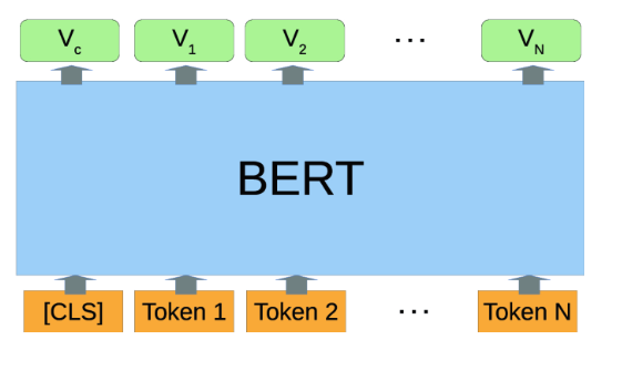
The main advantage of BERT is that it provides context-aware embeddings and also provides an embedding to our whole sentence. To learn the full details of implementing BERT, we’ll need knowledge of transformers and attention, which we will talk about in the future, but is unfortunately out of scope for this blog post, so we’ll just stick to this high-level explanation for now.

Conclusion:

In conclusion, word embeddings have revolutionized the way machines interpret human language, forming the backbone of modern Natural Language Processing (NLP) applications. Starting from the simplicity of one-hot encoding, where each word was represented in isolation, to the bag-of-words model that incorporated word frequency, early approaches provided foundational but limited insights into text meaning. The advent of models like Word2Vec and GloVe marked a turning point by embedding words in continuous vector spaces, allowing semantic similarities and relationships to be captured. This shift enabled models to understand context more effectively, improving tasks like sentiment analysis and machine translation. Finally, transformer-based models like BERT have pushed word embeddings further, representing words in a deeply contextualized manner by considering their surrounding text. This evolution not only captures nuanced meanings but also empowers NLP systems to handle complex language tasks with human-like proficiency. As NLP advances, word embeddings will continue to play a critical role, bridging the gap between human language and machine understanding.

Future of Word Embeddings:

The future of word embeddings in artificial intelligence is incredibly promising. We have moved from traditional techniques like Word2Vec and GloVe to cutting-edge models such as BERT and GPT, which capture the intricate relationships between words. These innovations not only improve text understanding but also enable the integration of diverse data types, including images, audio, and video, allowing AI systems to interpret information with greater precision. Furthermore, the rise of few-shot and zero-shot learning represents a significant leap toward developing adaptable AI models that can be generalized from limited examples. As we look ahead, it’s clear that these advancements will continue to shape the landscape of AI, fostering deeper and more meaningful interactions between humans and machines.